September 2023 I Volume 44, Issue 3
Review of Surrogate Strategies and Regularization with Application to High-Speed Flows
September 2023
Volume 44 I Issue 3
![]()
IN THIS JOURNAL:
- Issue at a Glance
- Chairman’s Message
Conversations with Experts
- Interview with Robert J. Arnold
Technical Articles
- I-TREE A Tool for Characterizing Research Using Taxonomies
- Scientific Measurement of Situation Awareness in Operational Testing
- Using ChangePoint Detection and AI to classify fuel pressure states in Aerial Refueling
- Post-hoc Uncertainty Quantification of Deep Learning Models Applied to Remote Sensing Image Scene Classification
- Development of Wald-Type and Score-Type Statistical Tests to Compare Live Test Data and Simulation Predictions
- Test and Evaluation of Systems with Embedded Machine Learning Components
- Experimental Design for Operational Utility
- Review of Surrogate Strategies and Regularization with Application to High-Speed Flows
- Estimating Sparsely and Irregularly Observed Multivariate Functional Data
- Statistical Methods Development Work for M and S Validation
News
- Association News
- Chapter News
- Corporate Member News
Review of Surrogate Strategies and Regularization with Application to High-Speed Flows

Dr. Gregory Hunt
Assistant Professor, Department of Mathematics, Williamsburg, VA
![]()

Dr. Robin Hunt
Research Aerospace Engineer, Hypersonic Airbreathing Propulsion Branch, NASA Langley Research Center, Hampton, VA
![]()
 Christopher D. Marley
Aerospace Engineer, Vehicle Analysis Branch, NASA Langley Research Center, Hampton, VA
Abstract
Surrogate modeling, also known as meta-modeling or emulation, is an important class of techniques used to reduce the burden of resource-intensive computational models by creating efficient and accurate approximations. Surrogates have been used to great effect in design, optimization, exploration, and uncertainty quantification for a range of problems. Consequently, the development, analysis, and practice of surrogate modeling is of broad interest. In this work, select surrogate modeling strategies are studied as archetypes in a discussion on parametric/nonparametric strategies, local/global modeling, complexity regularization, uncertainty quantification, and strengths/weaknesses. In particular, we consider several variants of two powerful surrogate modeling strategies: polynomial chaos and Gaussian process regression. We evaluate these approaches on several synthetic benchmarks and real models of a hypersonic inlet and thermal protection system. Throughout, we analyze trade-offs that must be navigated to create accurate, flexible, and robust surrogates.
Keywords: surrogate modeling, meta-modeling, polynomial chaos, gaussian process regression
Introduction
Surrogate modeling, also known as meta-modeling or emulation, is an approach broadly used across science and engineering to substitute resource-intensive computational models with quicker approximations (Queipo et al. 2005; Forrester and Keane 2009). For example, aerospace applications include the design of high-speed combustors, optimization of vehicle geometry, modeling spacesuit impact damage, uncertainty quantification for hypersonics, reentry flows, commercial supersonics, and airfoil icing (Shenoy et al. 2019; West and Hosder 2015; Cole et al. 2023; West and Phillips 2020; DeGennaro, Rowley, and Martinelli 2015; DiGregorio, West, and Choi 2022; Weaver-Rosen et al. 2022). Consequently, the development, analysis, and practice of surrogate modeling is widely of interest. Surrogates are powerful because computational models can be resource intensive, requiring long compute times or specialized software/hardware. Compounding this, it is often desirable to run computations hundreds or thousands of times, e.g., to build a database over the parameter space or use Monte Carlo methods to propagate uncertainty (Shenoy et al. 2019; Sacks et al. 1989; Queipo et al. 2005; Forrester and Keane 2009; Hu et al. 2016; Baurle 2017). To reduce computational burden, surrogate approaches build an efficient approximation of the model using a small number of runs and techniques from statistics and machine learning. These surrogate approximations are then used in place of the original model (Sacks et al. 1989; Queipo et al. 2005; Forrester and Keane 2009).
This work focuses analysis on several variants of two powerful strategies widely used in practice: (1) polynomial chaos (PC), and (2) Gaussian process regression (GPR) (Xiu and Karniadakis 2002; Gramacy 2020). Beyond the specifics, these archetypal methods help frame analysis of similar methods like, polynomial regression, kernel regression, radial basis function (RBF) interpolation, and support vector regression (Watson 1964; Fasshauer 2007; Drucker et al. 1996). Our analysis explores how surrogate strategies and regularization affect approximation efficiency and uncertainty quantification. After briefly reviewing the methods, we explore performance on a range of synthetic benchmarks and two real aerospace vignettes. Ultimately, as no surrogate strategy will always be the best, this work seeks to stimulate discussion on trade-offs among several widely-used approaches.
Polynomial Chaos: A Global Basis Expansion
Let η be the computational model that takes a d-dimensional input x=(x(1),…,x(d)) and outputs y=η(x). Polynomial chaos (PC) builds a surrogate ![]() as a linear combination of polynomials Ψi so that
as a linear combination of polynomials Ψi so that
where ![]() is a multivariate polynomial comprised of a product of 1-D polynomials
is a multivariate polynomial comprised of a product of 1-D polynomials ![]() and the
and the ![]() are learned from the data (see Sec. 2.1). Here, N is the number of polynomial terms so that
are learned from the data (see Sec. 2.1). Here, N is the number of polynomial terms so that ![]() is the ith polynomial in the expansion. (A nomenclature may be found at the end of the manuscript.) PC is a special case of polynomial regression and is thus a basis expansion using globally active elements
is the ith polynomial in the expansion. (A nomenclature may be found at the end of the manuscript.) PC is a special case of polynomial regression and is thus a basis expansion using globally active elements ![]() (x) which take on non-trivial values over the entire d-dimensional space. What differentiates PC from other polynomial models is moment-based quantities like the mean or variance may be simply calculated. Suppose we have a given desired input probability distribution ƒ. If one chooses the
(x) which take on non-trivial values over the entire d-dimensional space. What differentiates PC from other polynomial models is moment-based quantities like the mean or variance may be simply calculated. Suppose we have a given desired input probability distribution ƒ. If one chooses the ![]() to be orthonormal with respect ƒ, then if X∼ƒ and
to be orthonormal with respect ƒ, then if X∼ƒ and ![]() =
= ![]() (X) the mean μ(
(X) the mean μ(![]() ) and variance σ2(
) and variance σ2(![]() ) can be calculated from the fit coefficients as
) can be calculated from the fit coefficients as
(Xiu and Karniadakis 2002; Walters and Huyse 2002). This is a nice feature when the primary interest of surrogate modeling is tractably propagating uncertainty X∼ƒ through ![]() . For many common ƒ, implementations of corresponding
. For many common ƒ, implementations of corresponding ![]() exist in software (Xiu and Karniadakis 2002; Feinberg and Langtangen 2015).
exist in software (Xiu and Karniadakis 2002; Feinberg and Langtangen 2015).
Fitting and Regularizing PC
We consider data-driven approaches to estimating the ![]() from a sample of S training points X1,…,Xs and corresponding ys=η(xs ). Here each xs is a d-dimensional vector with corresponding real-valued output ys. In this work we consider several variants of least-squares regression. While other approaches exist, they often require specially choosing the xs, e.g., choosing them following a quadrature rule or sampling them randomly following particular distribution like f (Rosić and Diekmann 2015; Jones, Doostan, and Born 2013). Conversely, the regression approach produces estimates for any choice of xs. (Although, ideally the xs should be representative of the desired part of the input space). The simplest regression approach is ordinary least-squares (OLS) sometimes called “non-intrusive point collocation.” Here, the
from a sample of S training points X1,…,Xs and corresponding ys=η(xs ). Here each xs is a d-dimensional vector with corresponding real-valued output ys. In this work we consider several variants of least-squares regression. While other approaches exist, they often require specially choosing the xs, e.g., choosing them following a quadrature rule or sampling them randomly following particular distribution like f (Rosić and Diekmann 2015; Jones, Doostan, and Born 2013). Conversely, the regression approach produces estimates for any choice of xs. (Although, ideally the xs should be representative of the desired part of the input space). The simplest regression approach is ordinary least-squares (OLS) sometimes called “non-intrusive point collocation.” Here, the ![]() are estimated as the regression coefficients of regressing y onto Ψ0(x),…,Ψ(N-1)(x). If Ψ is the S×N design matrix with elements Ψsn = Ψ(n-1) (xs) and y=(y1,…,yS)T, then these OLS estimates are
are estimated as the regression coefficients of regressing y onto Ψ0(x),…,Ψ(N-1)(x). If Ψ is the S×N design matrix with elements Ψsn = Ψ(n-1) (xs) and y=(y1,…,yS)T, then these OLS estimates are
An important consideration is choosing which/how many ![]() to include. Including many higher-order
to include. Including many higher-order ![]() generally leads to a more flexible fit; however, it is prone to over-fitting where the complexity of the fit is not supported by enough training data. Over-fitting often leads to poor prediction accuracy in regions of the input space where the training data is sparse. Consequently, a primary fitting consideration is properly constraining model flexibility. This is known as model regularization. We consider three widely-used regularization approaches: (1) over-sampling, (2) ridge penalization, and (3) LASSO penalization.
generally leads to a more flexible fit; however, it is prone to over-fitting where the complexity of the fit is not supported by enough training data. Over-fitting often leads to poor prediction accuracy in regions of the input space where the training data is sparse. Consequently, a primary fitting consideration is properly constraining model flexibility. This is known as model regularization. We consider three widely-used regularization approaches: (1) over-sampling, (2) ridge penalization, and (3) LASSO penalization.

Figure 1. Comparing different OSR for a 5-dimensional input: (A) Number of polynomial terms in a PC model versus the sample size. Dashed lines are through the origin with slope 1/r where r=1,1.5,2. (B) Degree of polynomial fit versus the sample size.
Oversampling is the strategy whereby one includes only polynomials ![]() whose degree is less than or equal to some chosen integer P (Hosder, Walters, and Balch 2012). In the univariate case, this is exactly a Pth degree fit; for the multivariate case, this means only including terms where the sum of the degrees across the constituent univariate polynomials is at most P. Such models have
whose degree is less than or equal to some chosen integer P (Hosder, Walters, and Balch 2012). In the univariate case, this is exactly a Pth degree fit; for the multivariate case, this means only including terms where the sum of the degrees across the constituent univariate polynomials is at most P. Such models have  terms, which grows quickly in both d and P. To avoid over-fitting, modelers often employ over-sampling, capping N at some fraction
 ![]() of S so that there are at least r times as many training points as polynomial terms. Here, r is called the over-sampling ratio (OSR). Typically, this is done by choosing P as the largest integer where
of S so that there are at least r times as many training points as polynomial terms. Here, r is called the over-sampling ratio (OSR). Typically, this is done by choosing P as the largest integer where  (Hosder, Walters, and Balch 2012; West and Hosder 2015). Figure 1 displays the degree and number of terms in a five-dimensional example using OSR=1, 1.5, and 2 and a range of S. This figure helps visualize OSR limitations on the polynomial degree as the sample size increases.
Additionally, fit complexity may be regularized by explicit penalization. For example, ridge regression adds a L2 penalty to the least-squares loss L(w)=||Ψw-y||2 defining estimates as

for a regularization strength parameter λ>0 typically chosen via cross-validation (Hastie, Tibshirani, and Friedman 2001). Briefly, ridge posits that ![]() with very large values in the components correspond to very flexible fits and, conversely, fits are simpler as
with very large values in the components correspond to very flexible fits and, conversely, fits are simpler as ![]() →0. Thus ridge penalizes the typical OLS fit to avoid large values of
→0. Thus ridge penalizes the typical OLS fit to avoid large values of ![]() corresponding to overly-flexible fits (Hoerl and Kennard 1970a, 1970b). The parameter λ balances the trade-off between making L small and making
corresponding to overly-flexible fits (Hoerl and Kennard 1970a, 1970b). The parameter λ balances the trade-off between making L small and making ![]() small. Ridge estimates have a closed form solution
small. Ridge estimates have a closed form solution  . In a precise statistical sense, ridge reduces model complexity (degrees of freedom). For example, given orthonormal Ψ, ridge reduces the degrees of freedom from N to N/(1+λ) (Hoerl and Kennard 1970a, 1970b; Hastie, Tibshirani, and Friedman 2001).
Alternatively, the least absolute shrinkage and selection operator (LASSO) penalizes using a L1 penalty ![]() so the estimates are
so the estimates are
This penalty also discourages too much flexibility. Unlike ridge, LASSO also exactly zeros out elements of ![]() (LASSO) effectively removing the corresponding terms from the model (Tibshirani 1996). This is effectively a continuous approximation to the best-variable selection problem. LASSO is closely related to least-angle regression (LAR) or basis pursuit denoising (BPDN) (Chen, Donoho, and Saunders 2001; Efron et al. 2004). Since one still needs to choose N for a ridge/LASSO model, OSR rules are often used in combination with ridge/LASSO.
(LASSO) effectively removing the corresponding terms from the model (Tibshirani 1996). This is effectively a continuous approximation to the best-variable selection problem. LASSO is closely related to least-angle regression (LAR) or basis pursuit denoising (BPDN) (Chen, Donoho, and Saunders 2001; Efron et al. 2004). Since one still needs to choose N for a ridge/LASSO model, OSR rules are often used in combination with ridge/LASSO.
Gaussian Process Regression: A Localized Expansion
Radial basis function (RBF) GPR forms ![]() as a linear combination of RBFs
as a linear combination of RBFs  with tuning parameters τ2 and δ so that
for weights ![]() estimated from the training data (Gramacy 2020). The RBF functions are essentially Normal density functions with variances 1/(2δ), heights τ2, and means set to each of the training points xs. While RBF functions are a standard choice for the Ks, due to their locally constrained nature and ability to model smoothness, there are many other good choices (Duvenaud 2014). Figure 2 displays an example GPR fit.
estimated from the training data (Gramacy 2020). The RBF functions are essentially Normal density functions with variances 1/(2δ), heights τ2, and means set to each of the training points xs. While RBF functions are a standard choice for the Ks, due to their locally constrained nature and ability to model smoothness, there are many other good choices (Duvenaud 2014). Figure 2 displays an example GPR fit.

Figure 2. Example GPR Fit. Solid black curve is the true function η(x)=exp(xcos(2πx)) while solid red curve indicates GPR fit ![]() (x). Black dots indicate training points. Dashed red lines show the scaled RBF functions
(x). Black dots indicate training points. Dashed red lines show the scaled RBF functions ![]() Ks(x) whose sum forms
Ks(x) whose sum forms ![]() (x). Red dots indicate centers of the RBF curves corresponding to the training points.
(x). Red dots indicate centers of the RBF curves corresponding to the training points.
Fitting and Regularizing GPR
To fit GPR, one needs to identify weights ![]() 1,…,
1,…,![]() S and tuning parameters δ and τ2. If R is the S×S kernel matrix
S and tuning parameters δ and τ2. If R is the S×S kernel matrix  for training points xs and xs‘, then
 ![]() is typically estimated as
is typically estimated as
where ε is a smoothing parameter. If ε=0 the GPR interpolates the training data. For ε>0 it smooths over the data with higher ε inducing more smoothing. While sometimes perfectly interpolating the training data using GPR is warranted, if η is very complex or noisy, then interpolation can over-fit and better fits may be obtained via smoothing, even if η is deterministic.
The primary goal of fitting GPR is choosing good values for δ, τ2, and ε. Tuning δ sets the local adaptability with small values being less smooth and more locally adaptive, and large values conversely. Tuning ε can be understood as properly regularizing the balance between smoothing and interpolation. Tuning τ2 does not directly affect predictions, but tuning it can make numerical optimization more robust to finding good values for δ and ε. In particular, we determine δ, τ2, and ε via maximum likelihood estimation (MLE), which assumes a Gaussian process data-generating model and maximizes the resulting likelihood. In addition to providing estimates, GPR can provide confidence bands for ![]() (Gramacy 2020). Note, however, that these confidence bands come from a model where x is deterministic and η random; this is different than UQ otherwise discussed in this work, which assumes η is deterministic and x is random.
(Gramacy 2020). Note, however, that these confidence bands come from a model where x is deterministic and η random; this is different than UQ otherwise discussed in this work, which assumes η is deterministic and x is random.

Figure 3. Local GPR fit (left) and non-local polynomial fit (right) for two data sets. For the first data set, x values are evenly spaced over 0 to 1 and the y values are generated following η(x)=exp(xcos(2πx)). The second data set changes a single point in the training data.
Comparison of PC and GPR Model Forms
GPR and PC both form ![]() as a linear combination of functions with weights learned from the data. The
as a linear combination of functions with weights learned from the data. The ![]() used by PC have a global reach; they take on non-trivial values over the entire space and go to ±∞ as x→±∞. Conversely, the RBF Ks used by GPR have a local reach and exponentially decay to 0 as x moves away from xs, i.e.
used by PC have a global reach; they take on non-trivial values over the entire space and go to ±∞ as x→±∞. Conversely, the RBF Ks used by GPR have a local reach and exponentially decay to 0 as x moves away from xs, i.e. ![]() . Thus, each
. Thus, each ![]() influences predictions globally across all x while the influence of Ks is only locally near xs. Often, GPR can more easily fit bumpy functions where the values in one part of the space are largely de-coupled from those far away. Typically, PC does this less readily as choosing the correct linear combination of
influences predictions globally across all x while the influence of Ks is only locally near xs. Often, GPR can more easily fit bumpy functions where the values in one part of the space are largely de-coupled from those far away. Typically, PC does this less readily as choosing the correct linear combination of ![]() to create a bump in one part of the space often affects the predictions far away. As an example, Figure 3 displays 1D fits of GPR and PC for two synthetic data sets with/without a localized bump. Here, GPR readily adapts to the bump. The nature of PC and GPR also influences scaling and regularization of model complexity as the sample size grows. This is key to avoiding under-/over-fitting. GPR regularizes via a natively nonparametric framework, adding a Ks for each training point and then tuning δ/ε. PC can be retrospectively regularized using a non-parametric-like procedure by adding polynomial terms as the sample size grows, e.g., following an OSR rule and then adaptively regularizing via ridge/LASSO.
to create a bump in one part of the space often affects the predictions far away. As an example, Figure 3 displays 1D fits of GPR and PC for two synthetic data sets with/without a localized bump. Here, GPR readily adapts to the bump. The nature of PC and GPR also influences scaling and regularization of model complexity as the sample size grows. This is key to avoiding under-/over-fitting. GPR regularizes via a natively nonparametric framework, adding a Ks for each training point and then tuning δ/ε. PC can be retrospectively regularized using a non-parametric-like procedure by adding polynomial terms as the sample size grows, e.g., following an OSR rule and then adaptively regularizing via ridge/LASSO.
Reconstructing Synthetic Test Functions
We evaluate several surrogate modeling methods using numerical experiments on synthetic η, which allows evaluation in a context where the true complexity of η is known and controllable. We consider four surrogates: (1) GPR, (2) OLS PC, (3) ridge regularized PC, and (4) LASSO regularized PC. The PC methods are fit using both a low and high OSR regularization regime outlined in Table 1. All of the numerical experiments follow the same fitting and evaluation procedure using a Latin Hypercube Sampling (LHS) design for the training xs and then evaluation on an independent test grid of 100,000 points. While we may not have a test set in a real application (and might instead use cross-validation), our η are intentionally computationally inexpensive so a test set can be generated, thus providing an error metric with a simple interpretation. The same training/testing data are used across methods. We summarize error using median absolute error (MAE).
| Regime | OLS | ridge | LASSO |
| Low OSR | OSR=1 | OSR=1 | OSR=1 |
| High OSR | OSR=2 | OSR=1.5 | OSR=1.5 |
Table 1. Low and high OSR regularization regimes for PC methods. The high regime uses a lower OSR for ridge and LASSO as these have additional stabilizing regularization.

Figure 4. (A) Table of polynomial test functions considered. L1,…,LK are multivariate Legendre polynomials of total degree 10 or less and ak arbitrarily chosen between 0 and 1. Functions are rescaled using the displayed transformations so that the interesting part of the functions are in the unit hypercube. (B) 2D slices of test polynomials for a d=5 dimensional case. To standardize fitting and comparison, the x variables are re-scaled to be between zero and one (for each coordinate) and the y values are scaled to be between -1 and 1.
Polynomial Test Functions
We first consider performance of the surrogates on several five-dimensional polynomial test functions outlined in Figure 4 (A) with 2D slices of the functions visualized in subplot (B). Figure 5 displays MAE(![]() ) as the number of training points S varies. For each value of S, the numerical experiment is repeated 50/√S times. This repetition helps capture the range of potential fits over possible training datasets generated by the randomized LHS. (Fewer repetitions are needed for larger S as these fits are more stable.) Figure 5 demonstrates the need for regularization, as the error spikes for some of the fits, especially in the low OSR regime. Over-fitting risk is higher for less regularized approaches like OLS. Over-fitting susceptibility is also worse for more complicated η like the Styblinski-Tang and Legendre polynomials. Even though these functions are deterministic, the high level of complexity that cannot be captured by the models effectively acts as a “deterministic noise” and methods can overfit this “noise.” Increasing the level of OSR regularization (top v. bottom rows of Figure 5) significantly attenuates over-fitting. Furthermore, ridge and LASSO can help solve this problem by adaptively modifying the regularization, which lessens the dependence on OSR.
) as the number of training points S varies. For each value of S, the numerical experiment is repeated 50/√S times. This repetition helps capture the range of potential fits over possible training datasets generated by the randomized LHS. (Fewer repetitions are needed for larger S as these fits are more stable.) Figure 5 demonstrates the need for regularization, as the error spikes for some of the fits, especially in the low OSR regime. Over-fitting risk is higher for less regularized approaches like OLS. Over-fitting susceptibility is also worse for more complicated η like the Styblinski-Tang and Legendre polynomials. Even though these functions are deterministic, the high level of complexity that cannot be captured by the models effectively acts as a “deterministic noise” and methods can overfit this “noise.” Increasing the level of OSR regularization (top v. bottom rows of Figure 5) significantly attenuates over-fitting. Furthermore, ridge and LASSO can help solve this problem by adaptively modifying the regularization, which lessens the dependence on OSR.

Figure 5. MAE over a quasi-exponentially-spaced sequence of training points. For each value of S, the numerical experiment is repeated 50/√S times. The lines indicate the median MAE and shaded regions indicate the 25th and 75th percentiles of MAE. The top and bottom rows of plots correspond to the low and high OSR cases for PC methods, respectively.
Figure 5 also allows comparison of method error. For small S, the methods often perform similarly. Nonetheless, for low OSR, the PC error often decreases quicker than GPR as S increases, e.g., for the Styblinski-Tang, Rosenbrock, and bowl polynomials. Likely, this happens because PC is fitting a polynomial ![]() to a polynomial η. Consequently, by adding polynomial terms as S increases, we can often eventually fit the polynomial functions perfectly with PC. For example, the Styblinski-Tang and Rosenbrock functions are fourth-degree polynomials. When OSR=1 and S≥126, the PC methods perfectly fit 4th degree models. Similarly, for the bowl polynomial when OSR=1 and S≥21. This does not happen for the Legendre polynomial as we never consider a large enough S to perfectly fit a 10th degree polynomial and thus GPR performs relatively well. This result is sometimes sensitive to precise tuning of complexity via OSR. For example, moving to the high OSR-regime, PC methods sometimes fail to out-perform GPR even for large S, e.g., for the simple bowl polynomial. For small/medium S, the primary driver of accuracy seems to be the strategy to tune complexity to the amount of training data, e.g., with OSR, ridge/LASSO, or a non-parametric GPR fit. Surprisingly, PC does not always do this the best for truly polynomial η.
to a polynomial η. Consequently, by adding polynomial terms as S increases, we can often eventually fit the polynomial functions perfectly with PC. For example, the Styblinski-Tang and Rosenbrock functions are fourth-degree polynomials. When OSR=1 and S≥126, the PC methods perfectly fit 4th degree models. Similarly, for the bowl polynomial when OSR=1 and S≥21. This does not happen for the Legendre polynomial as we never consider a large enough S to perfectly fit a 10th degree polynomial and thus GPR performs relatively well. This result is sometimes sensitive to precise tuning of complexity via OSR. For example, moving to the high OSR-regime, PC methods sometimes fail to out-perform GPR even for large S, e.g., for the simple bowl polynomial. For small/medium S, the primary driver of accuracy seems to be the strategy to tune complexity to the amount of training data, e.g., with OSR, ridge/LASSO, or a non-parametric GPR fit. Surprisingly, PC does not always do this the best for truly polynomial η.

Figure 6. (A) Table of the bump test functions considered. Again, we use a d=5 dimensional space. For the Gaussian bumps we choose constants a1=15,a2=20,b1=1/3,b2=2/3. For the quadratic bumps we choose c=100,e1=1/4,e2=(1/2,2/3,…,d/(d+1)). (B) 2D slices of the bump functions. (C) MAE plotted over S.
Non-Polynomial Test Functions
We also evaluate the approaches on a series of non-polynomial test functions. First, we evaluate the methods on two types of “bump” functions displayed in Figure 6 that decay moving away from the center of the space. Figure 6 (C) displays MAE(![]() ) over S. Many of the previous observations still apply. For example, the less-regularized approaches risk over-fiting with spiking error, higher OSR and penalization helps attenuate this.
) over S. Many of the previous observations still apply. For example, the less-regularized approaches risk over-fiting with spiking error, higher OSR and penalization helps attenuate this.
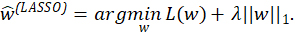
Figure 7. Example 2D slices of the truth and surrogate fits for the Gaussian bump function at S=500: (A) slice in the middle of the space where x3=x4=x5=1/2; (B) slice near the edge of the space where x3=x4=x5=1/10.
While none of the surrogates produce particularly accurate models until S is bigger than about 50, GPR seems to do quite well. This is expected, as the ability to model local features/bumps is built-in to GPR.
While MAE summarizes accuracy over the entire 5D space, no surrogate is uniformly accurate. Figure 7 investigates how accuracy is spatially-dependent with plots of 2D slices of the PC/GPR fits for the Gaussian bumps at S=500 and OSR=1. Subplot (A) shows a slice through the center of the region, (B) shows a slice near the edge. Considering (A), GPR does well and, somewhat counter-intuitively, so does OLS PC. The OLS PC captures the peanut-shape of the function well so long as we stay away from the edges. This is interesting, as OLS/OSR=1 has a substantially higher MAE than the other PC methods in Figure 6 (C). Notably, in subplot (B) OLS PC does less well comparatively. This happens because near the edges the OLS fit has not properly tuned complexity to the amount of training data and is over-fitting.
This edge-effect is quite general whereby very flexible fits will do well in the middle of the space at the expense of accuracy near the edges. This happens because in the middle of the space the fits are closer to more of the training points (on average) and so they have a lot of training data to properly support fitting a flexible model. Towards the edges of the space, the low data density cannot support the high flexibility. Essentially, very flexible methods trade-off higher accuracy in the middle of the space for less accuracy near the edges. Note that this tradeoff is only possible if η is sufficiently complex to warrant a complex fit. GPR can partially avoid this trade-off by using a more locally-adaptive approach to decouple the surrogate fit in the middle of the space from the edges and it does correspondingly well in all cases in Figure 6.

Figure 8. (A) Table of the trigonometric test functions considered. (B) 2D slices of the trigonometric test functions. (C) MAE plotted over S.
We conclude this section by considering method performance on three 5D trigonometric examples (Figure 8) that are neither polynomials nor specifically bumps and thus should not particularly favor either approach. Subplot (C) displays MAE over S, and we find consistent results with the previous examples. Well-regularized approaches like GPR and ridge/LASSO PC tend to perform quite well as compared to less regularized approaches – especially for very complex bumpy functions like the Trig. Prod. For simpler and smoother functions like the Trig. Sum or Hyper. Tan, GPR often performs well, however any of the PC approaches are highly competitive. The potential flexibility of a low OSR PC regularized by the adaptive data-driven ridge/LASSO is often very accurate in these cases.

Figure 9. Scamjet inlet model. (A) Schematic of the scramjet inlet. (B) 2D slice of η over θ1 and θ2 (where θ3=θ4=10∘). (C) MAE plotted over S.
Vignette: Modeling Total Pressure Recovery in High- Speed Inlet
As an example of surrogate modeling applied to an aerodynamic problem, this section explores a short vignette of modeling a scramjet inlet. The inlet is composed of four angled ramps, each of which creates an oblique shock. The flowfield properties are calculated across each shock assuming a calorically perfect gas and inviscid flow. This keeps computational expense low so that we may evaluate the model hundreds of times to comprehensively investigate accuracy. In particular, given the upstream Mach number normal to the shock M and relative ramp angle θ, the oblique shock wave angle β is calculated using the the well-known oblique shock β-θ-M relation (Anderson, J. D., Jr. 2011). Thus, the flow properties behind each shock can be calculated iteratively based on their pre-shock values. The goal in this example is to evaluate the inlet total pressure loss across a wide range of ramp angles. A schematic of the inlet is displayed in Figure 9 (A) and a 2D slice of η is displayed in subplot (B). Here, the input to the model η is the four ramp angles θ1,…,θ4 and the output is the total pressure ratio at the start of the inlet Pratio. To provide a broad range of configurations, the angles are varied over the range 0 to 35∘ with the constraint that the angles sum to less than 90∘. This leads to a non-square region in Figure 9 (B). Note the shape of η in this subplot is somewhat quadratic as a function of the θs. The value of Pratio over θ1 and θ2 appears somewhat similar to a second-degree bowl shaped function with a maximum near 5∘.
Figure 9 (C) shows the reconstruction accuracy of the various surrogate approaches ![]() in reconstructing the inlet model η. The behavior in this real problem mimics the behavior observed in the synthetic test functions. In the low OSR case, the ridge and LASSO penalized PC models also do quite well and are competitive with GPR. The high OSR case over-restricts the PC model complexity leading to a bigger performance gap. In both OSR regimes, the PC error drops significantly once second-degree terms are included (S≥15 for OSR=1). This comports with our observation that the surrogate η is well-approximated by a quadratic. Nonetheless, GPR is able to squeeze out some performance since it does need to fit a truly second-degree model.
in reconstructing the inlet model η. The behavior in this real problem mimics the behavior observed in the synthetic test functions. In the low OSR case, the ridge and LASSO penalized PC models also do quite well and are competitive with GPR. The high OSR case over-restricts the PC model complexity leading to a bigger performance gap. In both OSR regimes, the PC error drops significantly once second-degree terms are included (S≥15 for OSR=1). This comports with our observation that the surrogate η is well-approximated by a quadratic. Nonetheless, GPR is able to squeeze out some performance since it does need to fit a truly second-degree model.
Uncertainty Propagation
Assuming that X∼ƒ, this section compares the true uncertainty of Y=η(X) to the estimated uncertainty of ![]() =
= ![]() (X). To calculate accuracy using a universally applicable approach, we consider propagated mean/s.d. using Monte Carlo (MC) methods. We generate a new independent sample of 5,000 MC observations following ƒ, propagate them through
(X). To calculate accuracy using a universally applicable approach, we consider propagated mean/s.d. using Monte Carlo (MC) methods. We generate a new independent sample of 5,000 MC observations following ƒ, propagate them through ![]() , and calculate the resulting mean/s.d. The error is quantified as the absolute error of MC estimates compared to the true mean/s.d. For the PC methods, we also use the closed-form formulas for the mean/s.d. based on the fit coefficients and similarly calculate error. Additionally, for the MC approaches, we calculate the Wasserstein distance W as
, and calculate the resulting mean/s.d. The error is quantified as the absolute error of MC estimates compared to the true mean/s.d. For the PC methods, we also use the closed-form formulas for the mean/s.d. based on the fit coefficients and similarly calculate error. Additionally, for the MC approaches, we calculate the Wasserstein distance W as

where  are the true/estimated means/s.d.s and ν is the correlation between the true/estimated quantiles (Barrio, Giné, and Matrán 1999). The Wasserstein distance more holistically captures distribution differences (beyond mean/s.d.) by essentially capturing an “earth-mover’s” distance measuring the minimum amount of work needed to transform the true and surrogate distributions into one-another (Barrio, Giné, and Matrán 1999). In this section, we consider components of X independently following a Normal distribution with mean of 1/2 and standard deviation of 1/8 so that X falls between zero and one with high probability.
Figure 10 explores UQ accuracy for the Gaussian bumps. Notably, the difference between the MC approach (dashed lines) and coefficient approach (solid lines) is negligible showing that MC error is small. This is not an artifact the Gaussian bumps, but is true of all our examples. The accuracy of the UQ depends much more on the particular surrogate method ![]() than whether we use MC or the PC coefficient approach. Furthermore, since the surrogates are extremely fast to compute and generating 5000 MC observations is not burdensome, we can propagate the uncertainty in about 40ms on our standard 4GHz desktop. While the overall accuracy of GPR was often the lowest for the Gaussian bumps (c.f. Figure 6), the lowly-regularized OLS PC is often competitive with GPR in UQ accuracy (especially in the low OSR case). This happens due to the normal distribution of X which concentrates density (and MC observations) near the center of the space. This advantages very flexible fits that often do well in the middle of the space at the expense of accuracy near the edges (c.f. Figure 7). Previously, MAE was calculated on a test set uniformly distributed over the input space which reflected poor performance near the edges. Conversely, Figure 10 use points highly concentrated into the middle of the space which reflects the good performance of OLS with OSR=1 in this region.
than whether we use MC or the PC coefficient approach. Furthermore, since the surrogates are extremely fast to compute and generating 5000 MC observations is not burdensome, we can propagate the uncertainty in about 40ms on our standard 4GHz desktop. While the overall accuracy of GPR was often the lowest for the Gaussian bumps (c.f. Figure 6), the lowly-regularized OLS PC is often competitive with GPR in UQ accuracy (especially in the low OSR case). This happens due to the normal distribution of X which concentrates density (and MC observations) near the center of the space. This advantages very flexible fits that often do well in the middle of the space at the expense of accuracy near the edges (c.f. Figure 7). Previously, MAE was calculated on a test set uniformly distributed over the input space which reflected poor performance near the edges. Conversely, Figure 10 use points highly concentrated into the middle of the space which reflects the good performance of OLS with OSR=1 in this region.

Figure 10. Accuracy of propagated mean and s.d. for the Gaussian bump function. Lines indicate the median, shaded regions delineate 25th and 75th percentiles. Solid lines indicate PC coefficient approach, dashed-lines indicate MC approaches.
This is a general phenomena that will happen when the distribution of X is highly concentrated around the middle of the space. To explore this, Figure 11 displays the Wasserstein distance for several of the complex test functions. First consider the high OSR regime where the PC methods are more regularized to balance performance broadly across the entire space. For this bottom row of Figure 11, GPR is broadly more accurate than the PC methods and thus it tends to propagate uncertainty more accurately. However, in the low OSR case (top row of Figure 11), the extreme flexibility afforded to the OLS method allows it to sometimes be competitive with GPR. There is less of a difference for the ridge/LASSO methods which adaptively avoid over-fitting in all cases. Note, however, that this desirable behavior of OLS will only manifest if η is sufficiently complex to warrant a very flexible fit (at least in the middle of the space). This benefit disappears if η is a less complex function as demonstrated in Figure 12 which displays similar results for several of the simpler test functions. Here, the OLS with OSR=1 fit yields no particular dividends. Aside from this particular quirk for OLS, accuracy propagating uncertainty in Figure 11 and 12 seems to broadly follow overall surrogate accuracy as observed previously. This again emphasizes that UQ accuracy more closely follows the general accuracy of the surrogate ![]() than the particular UQ method (e.g. PC coefficient methods v. Monte Carlo).
than the particular UQ method (e.g. PC coefficient methods v. Monte Carlo).

Figure 11. Wasserstein distance for several complex test functions over values of S. Top row is low OSR, bottom row is high OSR.
 Figure 12. Wasserstein distance for several simple test functions over values of S. Top row is low OSR, bottom row is high OSR.
Vignette: Uncertainty Propagation for a Thermal Protection System

Figure 13. Schematic of a passive thermal protection system architecture comprised of a space shuttle ceramic tile and a titanium 6242 facesheet.
Passive Thermal Protection Systems (TPS) are an important component of many high-speed vehicles such as space launch or reentry vehicles. In this section, we model a TPS with the goal of studying how design parameters affect prevention of the TPS temperature exceeding a target over a fixed time. The model TPS is comprised of a ceramic tile with a titanium facesheet as displayed in Figure 13. The ceramic tile and facesheet have thicknesses htile and hTi. Exposure to high speed flow leads energy qconv being transferred to the tile via heating. As energy is absorbed by the tile, the temperature of the outer wall, Tw, increases, causing energy to be radiated out, qrad. The net heat flux into the TPS is the difference between the convective heat flux in and the radiative heat flux out. Over time, as energy is continuously absorbed at the outer wall, the energy is conducted through the ceramic tile down to the titanium facesheet and the temperature of the titanium, TTi, increases. This temperature is modeled using the unsteady, one dimensional heat conduction equation (Lienhard 2020). This model is a function of many physical constants and design parameters. Among them, several important parameters are: ξ, is the emissivity of the tile outer surface, M∞, freestream Mach number, tfinal the exposure period, and F, a model correction factor when calculating the Nusselt number (Lienhard 2020).
To study the uncertainty of this TPS model, we propagate Normally distributed uncertainty of five input parameters (see Table 2) and observe the subsequent final titanium temperature TTi. The Wasserstein distance for the surrogates is displayed in Figure 14. These results confirm our simulation results. That is, for this straight-forward problem, UQ accuracy broadly follows previous trends in surrogate accuracy. Broadly, all of the PC approaches perform similarly, with the OLS suffering in the high-OSR regime as it does not scale up complexity quick enough and under-fits. Ridge/LASSO penalization seem to solve this issue and perform similarly in both regimes. The GPR approach performs quite well overall and is able increment complexity in a fine-tuned manner for small sample sizes. For S≥50, all methods perform well.
| Parameter | Mean | S.D. |
| htile | 0.0254 | 0.000635 |
| ξ | 0.8 | 0.025 |
| M∞ | 5.0 | 0.05 |
| F | 1.0 | 0.025 |
| tfinal | 60 | 1.25 |
Table 2. Input uncertainty distributions for parameters considered. Each parameter is assumed to follow a Normal distribution with the given mean and s.d.

Figure 14. Wasserstein distance for surrogates of the TPS model: (A) low OSR regime; (B) high OSR regime.
Conclusion
This work presents a comprehensive analysis of several variants of PC and GPR applied to real and synthetic examples. We expect much of the findings to generalize to other similar strategies. Overall, the accuracy and robustness of the surrogate modeling strategies is strongly tied to the ability of the approaches to properly regularize the complexity of the fits as the amount of training data increases either via a native non-parametric approach like GPR or an adaptively regularized parametric approach like PC with a reasonable OSR rule. GPR was relatively stronger for very bumpy functions while PC was often preferable when fitting polynomials. Directions for future work include building a theoretical understanding of how much like a polynomial the true computational model needs to be to lend an advantage to PC over GPR. This would likely benefit from rigorous definition of how “bumpy” a function is and how much a function resembles a polynomial.
This work considers problems with modest values of d, around d=5, as we demonstrated in our synthetic data examples. We expect this value of d to be relevant to many real-world aerodynamic problems. Nonetheless, for more complex, high-dimensional problems, all surrogate methods will face issues. One general approach to avoid this may be dimensionality reduction. Another may be to use specific methods which can partially resist the curse of dimensionality, like random forests (Breiman 2001). For uncertainty propagation, our results did not find that the PC coefficient approach was strongly preferable to MC propagation either in terms of accuracy of computational burden. An advantage of MC propagation is that it is quite general and imposes no special requirements on design, input uncertainties, or quantities of interest.
In closing, we again note that a key to surrogate modeling is to properly balance the trade-off between model flexibility and fit stability. There is no free lunch and no one method that will always perform the best. Data-driven regularization of fit complexity and flexibility is often quite good at navigating the space of models and matching a good surrogate to the computational model.
Nomenclature
Section 2.
| d | = dimension of input variable [11 scalar] |
| η | = true model [d1 function] |
| = surrogate model [d1 function] | |
| x | = generic input variable [d1 vector] |
| x(k) | = kth component of generic input variable [11 scalar] |
| X | = generic input variable (random) [d1 random vector] |
| X(k) | = kth generic component of input variable (random) [11 random scalar] |
| ƒ | = probability density function of X |
| xs | = sth training input [d1 vector] |
| S | = number of training samples [11 scalar] |
| y | = generic output variable [11 scalar] |
| Y | = generic output variable (random) [11 random scalar] |
| ys | = sth training output [11 scalar] |
| = surrogate output (random) [11 random scalar] | |
| μ(⋅) | = expected value (mean) [11 scalar] |
| σ2(⋅) | = variance [11 scalar] |
| i | = index of polynomial terms |
| = PC basis (multivariate) polynomial [d1 function] | |
| Ψik | = 1-D polynomial [11 function] |
| = ith PC weight [11 scalar] | |
| N | = num. PC polynomial terms [11 scalar] |
| Ψ | = matrix of PC polynomials evaluted on training data [SN matrix] |
| = OLS estimates of |
|
| = ridge estimates of |
|
| = LASSO estimates of |
|
| P | = maximum total degree of PC model [11 scalar] |
| r | = OSR ratio [11 scalar] |
| L | = least-squares loss |
| λ | = ridge or LASSO regularization strength [11 scalar] |
| ||⋅|| | = Euclidean norm (L2) |
| ||⋅||1 | = L1 norm |
Section 3
| Ks | = sth RBF function [d1 function] |
| τ2 | = scale for RBF function [11 scalar] |
| δ | = length-scale for RBF function [11 scalar] |
| = sth weight for GPR [11 scalar] | |
| R | = kernel matrix for GPR training observations [SS matrix] |
| ε | = smoothing/interpolation regularization parameter for GPR [11 scalar] |
| L | = likelihood function |
References
Anderson, J. D., Jr. 2011. Fundamentals of Aerodynamics. 5th ed. New York, NY, USA: McGraw-Hill.
Barrio, Eustasio del, Evarist Giné, and Carlos Matrán. 1999. “Central Limit Theorems for the Wasserstein Distance Between the Empirical and the True Distributions.” The Annals of Probability 27 (2): 1009–71. https://doi.org/10.1214/aop/1022677394.
Baurle, R. A. 2017. “Hybrid Reynolds-Averaged/Large-Eddy Simulation of a Scramjet Cavity Flameholder.” AIAA Journal 55 (2): 544–60. https://doi.org/10.2514/1.J055339.
Breiman, Leo. 2001. “Random Forests.” Machine Learning 45 (1): 5–32. https://doi.org/10.1023/a:1010933404324.
Chen, Scott Shaobing, David L. Donoho, and Michael A. Saunders. 2001. “Atomic Decomposition by Basis Pursuit.” SIAM Review 43 (1): 129–59. http://www.jstor.org/stable/3649687.
Cole, D. Austin, Robert B. Gramacy, James E. Warner, Geoffrey F. Bomarito, Patrick E. Leser, and William P. Leser. 2023. “Entropy-Based Adaptive Design for Contour Finding and Estimating Reliability.” Journal of Quality Technology 55 (1): 43–60. https://doi.org/10.1080/00224065.2022.2053795.
DeGennaro, Anthony M., Clarence W. Rowley, and Luigi Martinelli. 2015. “Uncertainty Quantification for Airfoil Icing Using Polynomial Chaos Expansions.” Journal of Aircraft 52 (5): 1404–11. https://doi.org/10.2514/1.C032698.
DiGregorio, N. J., T. K. West, and S. Choi. 2022. “Robust Design Under Uncertainty of Hypersonic Inlets.” In. AIAA Aviation 2022 Forum. https://doi.org/https://doi.org/10.2514/6.2022-3862.
Drucker, Harris, Christopher J. C. Burges, Linda Kaufman, Alex Smola, and Vladimir Vapnik. 1996. “Support Vector Regression Machines.” In Advances in Neural Information Processing Systems, edited by M. C. Mozer, M. Jordan, and T. Petsche. Vol. 9. MIT Press. https://proceedings.neurips.cc/paper/1996/file/d38901788c533e8286cb6400b40b386d-Paper.pdf.
Duvenaud, D. K. 2014. “Automatic Model Construction with Gaussian Processes.” PhD thesis, University of Cambridge. https://doi.org/10.17863/CAM.14087.
Efron, Bradley, Trevor Hastie, Iain Johnstone, and Robert Tibshirani. 2004. “Least angle regression.” The Annals of Statistics 32 (2): 407–99. https://doi.org/10.1214/009053604000000067.
Fasshauer, Gregory E. 2007. Meshfree Approximation Methods with Matlab. WORLD SCIENTIFIC. https://doi.org/10.1142/6437.
Feinberg, Jonathan, and Hans Petter Langtangen. 2015. “Chaospy: An Open Source Tool for Designing Methods of Uncertainty Quantification.” Journal of Computational Science 11: 46–57. https://doi.org/10.1016/j.jocs.2015.08.008.
Forrester, Alexander I. J., and Andy J. Keane. 2009. “Recent Advances in Surrogate-Based Optimization.” Progress in Aerospace Sciences 45 (1): 50–79. https://doi.org/10.1016/j.paerosci.2008.11.001.
Gramacy, Robert B. 2020. Surrogates: Gaussian Process Modeling, Design and Optimization for the Applied Sciences. Boca Raton, FL, USA: Chapman Hall/CRC. http://bobby.gramacy.com/surrogates/.
Hastie, Trevor, Robert Tibshirani, and Jerome Friedman. 2001. The Elements of Statistical Learning. Springer Series in Statistics. New York, NY, USA: Springer. https://doi.org/10.1007/978-0-387-84858-7.
Hoerl, Arthur E., and Robert W. Kennard. 1970a. “Ridge Regression: Applications to Nonorthogonal Problems.” Technometrics 12 (1): 69–82. https://doi.org/10.1080/00401706.1970.10488635.
Hoerl, Arthur E., and Robert W. Kennard. 1970b. “Ridge Regression: Biased Estimation for Nonorthogonal Problems.” Technometrics 12 (1): 55–67. https://doi.org/10.1080/00401706.1970.10488634.
Hosder, Serhat, Robert Walters, and Michael Balch. 2012. “Efficient Sampling for Non-Intrusive Polynomial Chaos Applications with Multiple Uncertain Input Variables.” https://doi.org/10.2514/6.2007-1939.
Hu, Xingzhi, Xiaoqian Chen, Geoffrey T. Parks, and Wen Yao. 2016. “Review of Improved Monte Carlo Methods in Uncertainty-Based Design Optimization for Aerospace Vehicles.” Progress in Aerospace Sciences 86: 20–27. https://doi.org/10.1016/j.paerosci.2016.07.004.
Jones, Brandon A., Alireza Doostan, and George H. Born. 2013. “Nonlinear Propagation of Orbit Uncertainty Using Non-Intrusive Polynomial Chaos.” Journal of Guidance, Control, and Dynamics 36 (2): 430–44. https://doi.org/10.2514/1.57599.
Lienhard, John H. 2020. “Heat Transfer in Flat-Plate Boundary Layers: A Correlation for Laminar, Transitional, and Turbulent Flow.” Journal of Heat Transfer. https://doi.org/10.1115/1.4046795.
Queipo, Nestor V., Raphael T. Haftka, Wei Shyy, Tushar Goel, Rajkumar Vaidyanathan, and P. Kevin Tucker. 2005. “Surrogate-Based Analysis and Optimization.” Progress in Aerospace Sciences 41 (1): 1–28. https://doi.org/10.1016/j.paerosci.2005.02.001.
Rosić, Bojana V., and Jobst H. Diekmann. 2015. “Methods for the Uncertainty Quantification of Aircraft Simulation Models.” Journal of Aircraft 52 (4): 1247–55. https://doi.org/10.2514/1.C032856.
Sacks, Jerome, William J. Welch, Toby J. Mitchell, and Henry P. Wynn. 1989. “Design and Analysis of Computer Experiments.” Statistical Science 4 (4): 409–23. https://doi.org/10.1214/ss/1177012413.
Shenoy, R. R., T. G. Drozda, R. A. Baurle, and P. A. Parker. 2019. “Surrogate Modeling and Optimization of a Combustor with an Interdigitated Flushwall Injector.” In. Programmatic; Industrial Base (PIB) Meeting. https://ntrs.nasa.gov/citations/20200002820.
Tibshirani, Robert. 1996. “Regression Shrinkage and Selection via the Lasso.” Journal of the Royal Statistical Society: Series B (Methodological) 58 (1): 267–88. https://doi.org/10.1111/j.2517-6161.1996.tb02080.x.
Walters, Robert W., and Luc Huyse. 2002. “Uncertainty Analysis for Fluid Mechanics with Applications.” In NASA/CR-2002-211449.
Watson, Geoffrey S. 1964. “Smooth Regression Analysis.” Sankhyā: The Indian Journal of Statistics, Series A (1961-2002) 26 (4): 359–72. http://www.jstor.org/stable/25049340.
Weaver-Rosen, J. M., Y.-K. Tsai, J. Schoppe, Y. Terada, R. Malak, P. G. A. Cizmas, and D. S. Lazzara. 2022. “Surrogate Modeling and Parametric Optimization Strategy for Minimizing Sonic Boom in a Morphing Aircraft.” In. AIAA Scitech 2022 Forum. https://doi.org/https://doi.org/10.2514/6.2022-0097.
West, Thomas K., and Serhat Hosder. 2015. “Uncertainty Quantification of Hypersonic Reentry Flows with Sparse Sampling and Stochastic Expansions.” Journal of Spacecraft and Rockets 52 (1): 120–33. https://doi.org/10.2514/1.A32947.
West, Thomas K., and Ben D. Phillips. 2020. “Multifidelity Uncertainty Quantification of a Commercial Supersonic Transport.” Journal of Aircraft 57 (3): 491–500. https://doi.org/10.2514/1.C035496.
Xiu, Dongbin, and George Em Karniadakis. 2002. “The Wiener–Askey Polynomial Chaos for Stochastic Differential Equations.” SIAM Journal on Scientific Computing 24 (2): 619–44. https://doi.org/10.1137/S1064827501387826.
Author Biography
Dr. Gregory Hunt is an assistant professor in the Department of Mathematics at the College of William & Mary. He is an interdisciplinary researcher that builds scientific tools. His formal training is in statistics, mathematics, and computer science. He works on a diverse set of problems in biology, physics, and engineering.
Dr. Robin Hunt is a research aerospace engineer in the Hypersonic Airbreathing Propulsion Branch at NASA Langley Research Center. Before joining NASA, she received her B.S. degree from the University of Maryland and M.S. and Ph.D. degrees from the University of Michigan.
Christopher D. Marley received his B.S. and M.S. from the Missouri University of Science and Technology and his Ph.D. from the University of Michigan. He worked as a hypersonic propulsion engineer at Boeing Research and Technology in Huntington Beach and as an aerothermodynamics engineer in the Vehicle Analysis Branch at NASA Langley.